ANNs with Keras#
To represent complex hypotheses with ANNs we need thousands or even millions of artificial neurons. ANNs with few large layers turned out be less effective than ANNs with many smaller layers. The latter are referred to as deep networks and their usage is known as deep learning.
Training ANNs requires lots of computation time for large data sets and large networks. Thus, we need efficient implementations of learning procedures and powerful hardware. Scikit-Learn aims at educational projects and offers a wide scale of machine learning methods. Implementation is less optimized for execution speed than for providing insight into the algorithms and providing access to all the parameters and intermediate results. Further, Scikit-Learn does not use all features of modern hardware.
Libraries for high-performance machine learning have to be more specialized on specific tasks to allow for optimizing efficiency. Keras is an open source library for implementing and training ANNs. Like Scikit-Learn it provides preprocessing routines as well as postprocessing (optimizing hyperparameters). But Keras utilizes full computation power of modern computers for training ANNs, leading to much shorter training times.
Modern computers have multi-core CPUs. So they can process several programs in parallel. In addition, almost all computers have a powerful GPU (graphics processing unit). It’s like a second CPU specialized at doing floating point computations for rendering 3d graphics. GPUs are much more suited for training ANNs than CPUs, because they are designed to work with many large matrices of floating point numbers in parallel. Nowadays GPUs can be accessed by software developers relatively easily. Thus, we may run programs on the GPU instead of the CPU.
Keras seamlessly integrates GPU power for ANN training into Python. We do not have to care about the details. Keras piggybacks on an open source library called TensorFlow developed by Google. Keras does much of the work for us, but from time to time TensorFlow will show up, too. Keras started independently from TensorFlow, then integrated support for TensorFlow, and now is distributed as a module in the TensorFlow Python package.
import tensorflow.keras as keras
2025-05-15 06:43:56.854757: I tensorflow/core/util/port.cc:153] oneDNN custom operations are on. You may see slightly different numerical results due to floating-point round-off errors from different computation orders. To turn them off, set the environment variable `TF_ENABLE_ONEDNN_OPTS=0`.
2025-05-15 06:43:56.865144: E external/local_xla/xla/stream_executor/cuda/cuda_fft.cc:477] Unable to register cuFFT factory: Attempting to register factory for plugin cuFFT when one has already been registered
WARNING: All log messages before absl::InitializeLog() is called are written to STDERR
E0000 00:00:1747284236.877630  953442 cuda_dnn.cc:8310] Unable to register cuDNN factory: Attempting to register factory for plugin cuDNN when one has already been registered
E0000 00:00:1747284236.881230  953442 cuda_blas.cc:1418] Unable to register cuBLAS factory: Attempting to register factory for plugin cuBLAS when one has already been registered
2025-05-15 06:43:56.893763: I tensorflow/core/platform/cpu_feature_guard.cc:210] This TensorFlow binary is optimized to use available CPU instructions in performance-critical operations.
To enable the following instructions: AVX2 AVX_VNNI FMA, in other operations, rebuild TensorFlow with the appropriate compiler flags.
An ANN for Handwritten Digit Recognition#
To demonstrate usage of Keras we implement and train a layered feedforward ANN to classify handwritten digits from the QMNIST data set. Inputs to the ANN are images of size 28x28. Thus, the feature space has dimension 784. Outputs are 10 real numbers in \([0,1]\). Each number represents the probability that the image shows the corresponding digit.
We could also use an ANN with only one output and require that this output is the digit, that is, it has range \([0,9]\). But how to interpret an output of 3.5? It suggests that the ANN cannot decide between 3 and 4. Or it might waffle on 2 and 5. Using only one output we would introduce artificial order and, thus, wrong similarity assumptions. From the view of similarity of shape (and only that matters in digit recognition), 3 and 8 are more close to each other than 7 and 8 are. Using one output per figure we avoid artificial assumptions and get more precise information on possible missclassifications. Images with high outputs for both 1 and 7 could be marked for subsequent review by a human, for example
Loading Data#
For loading QMNIST data we may reuse code from Load QMNIST project. We have to load training data and test data, both consisting of 60000 images and corresponding labels.
import matplotlib.pyplot as plt
import numpy as np
import pandas as pd
import seaborn as sns

import qmnist
train_images, train_labels, _, _ = qmnist.load('../../../../datasets/qmnist/', subset='train')
test_images, test_labels, _, _ = qmnist.load('../../../../datasets/qmnist/', subset='test')
train_images.shape, test_images.shape, train_labels.shape, test_labels.shape
((60000, 28, 28), (60000, 28, 28), (60000,), (60000,))
train_images[0, :, :].min(), train_images[0, :, :].max()
(np.float16(0.0), np.float16(1.0))
For visualization of data we use a gray scale with black at smallest value and white at highest value.
def show_image(img):
    fig, ax = plt.subplots(figsize=(2, 2))
    ax.imshow(img, vmin=0, vmax=1, cmap='gray')
    ax.axis('off')
    plt.show()
idx = 123

show_image(train_images[idx, :, :])
print('label:', train_labels[idx])

label: 7
Preprocessing#
Input to an ANN should be standardized or normalized. QMNIST images have range \([0, 1]\). That’s okay.
Optionally, we may center the images with respect to a figure’s bounding box. Without this step the center of mass is identical to the image center (we may reuse code from Image Processing with NumPy). As a by-product of centering bounding boxes each image will have 4 unused pixels at the boundary. Thus, we may crop images to 20x20 pixels without loss of information (resulting in 400 instead of 784 features).
def auto_crop(img):

    # binarize image
    mask = img > 0

    # whole image black?
    if not mask.any():
        return np.array([])

    # get top and bottom index of bounding box
    row_mask = mask.any(axis=1)
    top = np.argmax(row_mask)
    bottom = row_mask.size - np.argmax(row_mask[::-1])    # bottom index + 1

    # get left and right index of bounding box
    col_mask = mask[top:bottom, :].any(axis=0)    # [top:bottom, :] for efficiency only
    left = np.argmax(col_mask)
    right = col_mask.size - np.argmax(col_mask[::-1])    # right index + 1

    # crop
    return img[top:bottom, left:right].copy()


def center(img, n):

    # check image size
    if np.max(img.shape) > n:
        print('n too small! Cropping image.')
        img = img[0:np.minimum(n, img.shape[0]), 0:np.minimum(n, img.shape[1])]

    # calculate margin width
    top_margin = (n - img.shape[0]) // 2
    left_margin = (n - img.shape[1]) // 2

    # create image
    img_new = np.zeros((n, n), dtype=img.dtype)
    img_new[top_margin:(top_margin + img.shape[0]),
            left_margin:(left_margin + img.shape[1])] = img

    return img_new
train_images = qmnist.preprocess(train_images, [auto_crop, lambda img: center(img, 20)])
test_images = qmnist.preprocess(test_images, [auto_crop, lambda img: center(img, 20)])
idx = 123

show_image(train_images[idx, :, :])
print('label:', train_labels[idx])

label: 7
Training labels have to be one-hot encoded. This can be done manually with NumPy or automatically with Pandas or Scikit-Learn. Also Keras provides a function for one-hot encoding: to_categorical.
train_labels = keras.utils.to_categorical(train_labels)
test_labels = keras.utils.to_categorical(test_labels)

train_labels.shape, test_labels.shape
((60000, 10), (60000, 10))
Defining the ANN#
Keras has a Model class representing a directed graph of layers of neurons. At the moment we content ourselves with simple network structures, that is, we have a sequence of layers. For such simple structures Keras has the Sequential class. That class represents a stack of layers of neurons. It’s a subclass of Model.
A layer is represented by one of several layer classes in Keras. For a fully connected feedforward ANN we need an Input layer and several Dense layers. Layers can be added one by one with Sequential.add.
Input layers accept multi-dimensional inputs. Thus, we do not have to convert the 20x20 images to vectors with 400 components. But Dense layers want to have one-dimensional input. Thus, we use a Flatten layer. Like the Input layer that’s not a layer of neurons. Layers in Keras have to be understood as transformations taking some input and yielding some output. For Dense layers we need to specify the number of neurons and the activation function to use. There are several pre-defined activation functions in Keras.
Layers may have a name, which will help accessing single layers for analysis of a trained model. If we do not specify layer names, Keras generates them automatically.
model = keras.Sequential()

model.add(keras.Input(shape=(20, 20)))
model.add(keras.layers.Flatten())

model.add(keras.layers.Dense(10, activation='relu', name='dense1'))
model.add(keras.layers.Dense(10, activation='relu', name='dense2'))
2025-05-15 06:44:11.093713: E external/local_xla/xla/stream_executor/cuda/cuda_driver.cc:152] failed call to cuInit: INTERNAL: CUDA error: Failed call to cuInit: UNKNOWN ERROR (303)
The output layer is a Dense layer with 10 neurons. Because all outputs shall have range [0,1] we use the sigmoid function.
model.add(keras.layers.Dense(10, activation='sigmoid', name='out'))
Output shape can be accessed via corresponding member variable:
model.output_shape
(None, 10)
Almost always the first dimension of input or output shapes is the batch size for mini-batch training in Keras. None is used, if there is no fixed batch size.
More detailed information about the constructed ANN is provided by Sequential.summary:
model.summary()
Model: "sequential"
┏━━━━━━━━━━━━━━━━━━━━━━━━━━━━━━━━━┳━━━━━━━━━━━━━━━━━━━━━━━━┳━━━━━━━━━━━━━━━┓
┃ Layer (type)                    ┃ Output Shape           ┃       Param # ┃
┡━━━━━━━━━━━━━━━━━━━━━━━━━━━━━━━━━╇━━━━━━━━━━━━━━━━━━━━━━━━╇━━━━━━━━━━━━━━━┩
│ flatten (Flatten)               │ (None, 400)            │             0 │
├─────────────────────────────────┼────────────────────────┼───────────────┤
│ dense1 (Dense)                  │ (None, 10)             │         4,010 │
├─────────────────────────────────┼────────────────────────┼───────────────┤
│ dense2 (Dense)                  │ (None, 10)             │           110 │
├─────────────────────────────────┼────────────────────────┼───────────────┤
│ out (Dense)                     │ (None, 10)             │           110 │
└─────────────────────────────────┴────────────────────────┴───────────────┘
Total params: 4,230 (16.52 KB)
Trainable params: 4,230 (16.52 KB)
Non-trainable params: 0 (0.00 B)
Training the ANN#
Parameters for training are set with Model.compile. Here we may define an optimization routine. Next to gradient descent there are several other optimizers available. The optimizer can be passed by name (as string) or we may create a Python object of the respective optimizer class. The latter allows for custom parameter choice.
Next to the optimizer we have to provide a loss function. Again we may pass a string or an object. Because we have a classification problem we may use log loss.
If we want to validate the model during training, we may pass validation metrics to compile. Then output during training includes updated values for the validation metrics on training and validation data. For classification we may use accuracy score. Again, metrics can be passsed by name or as an object. Since we might wish to compute several different metrics, the metrics argument expects a list.
model.compile(optimizer='sgd', loss='categorical_crossentropy', metrics=['categorical_accuracy'])
Now the model is ready for training. In Keras training is done by calling Model.fit. We may specify the batch size for mini-batch training and the number of epochs. An epoch is a sequence of iterations required to cycle through the training data once. Small batch sizes require more iterations per epoch, large batch sizes require fewer iterations. In full-batch training epochs and iterations are equivalent. We may also specify validation data (directly or as fraction of the training data) to get validation metrics after each epoch. Thus, we can see wether the model overfits the data during training and abort training if necessary. The return value of fit will be discussed below.
history = model.fit(train_images, train_labels, batch_size=100, epochs=5, validation_split=0.2)
Epoch 1/5
480/480 ━━━━━━━━━━━━━━━━━━━━ 1s 2ms/step - categorical_accuracy: 0.2685 - loss: 2.1460 - val_categorical_accuracy: 0.5398 - val_loss: 1.5478
Epoch 2/5
480/480 ━━━━━━━━━━━━━━━━━━━━ 1s 2ms/step - categorical_accuracy: 0.5827 - loss: 1.3509 - val_categorical_accuracy: 0.7191 - val_loss: 0.8579
Epoch 3/5
480/480 ━━━━━━━━━━━━━━━━━━━━ 1s 2ms/step - categorical_accuracy: 0.7459 - loss: 0.8128 - val_categorical_accuracy: 0.8364 - val_loss: 0.5938
Epoch 4/5
480/480 ━━━━━━━━━━━━━━━━━━━━ 1s 2ms/step - categorical_accuracy: 0.8318 - loss: 0.5972 - val_categorical_accuracy: 0.8660 - val_loss: 0.4782
Epoch 5/5
480/480 ━━━━━━━━━━━━━━━━━━━━ 1s 2ms/step - categorical_accuracy: 0.8628 - loss: 0.4922 - val_categorical_accuracy: 0.8809 - val_loss: 0.4238
Hint
Note that validation accuracy displayed by Keras sometimes is higher than training accuracy. The reason is that train accuracy is the mean over all iterations of an epoche, but validation accuracy is calulated only at the end of an epoche. Thus, training accuracy includes poorer accuracy values from beginning of an epoche.
Incremental Training#
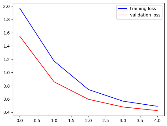
The Model.fit method returns a History object containing information about loss and metrics for each training epoch. The object has a dict member history containing losses and metrics. Loss keys are loss and val_loss for training and validation, respectively. Metrics keys depend an the chosen metrics.
fig, ax = plt.subplots()
ax.plot(history.history['loss'], '-b', label='training loss')
ax.plot(history.history['val_loss'], '-r', label='validation loss')
ax.legend()
plt.show()
fig, ax = plt.subplots()
ax.plot(history.history['categorical_accuracy'], '-b', label='training accuracy')
ax.plot(history.history['val_categorical_accuracy'], '-r', label='validation accuracy')
ax.legend()
plt.show()
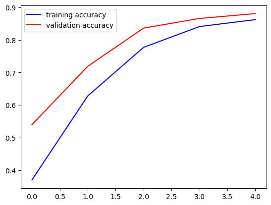
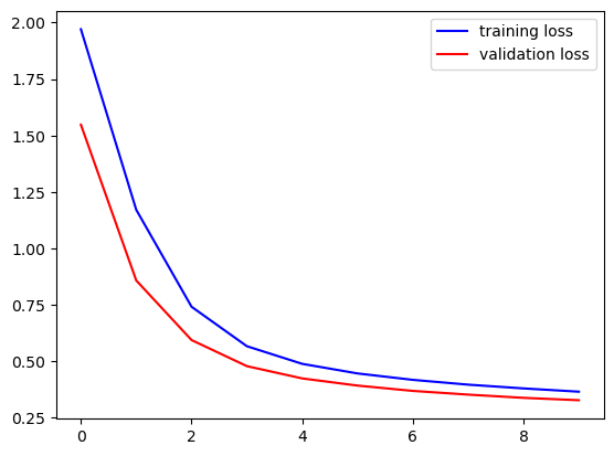
We see that further training could improve the model. Thus, we call fit again. Training proceeds from where it has been stopped. We may execute corresponding code cell as often as we like to continue training. To keep the losses and metrics we append them to lists.
loss = history.history['loss']
val_loss = history.history['val_loss']
acc = history.history['categorical_accuracy']
val_acc = history.history['val_categorical_accuracy']
history = model.fit(train_images, train_labels, batch_size=100, epochs=5, validation_split=0.2)

loss.extend(history.history['loss'])
val_loss.extend(history.history['val_loss'])
acc.extend(history.history['categorical_accuracy'])
val_acc.extend(history.history['val_categorical_accuracy'])
Epoch 1/5
480/480 ━━━━━━━━━━━━━━━━━━━━ 1s 2ms/step - categorical_accuracy: 0.8715 - loss: 0.4565 - val_categorical_accuracy: 0.8881 - val_loss: 0.3921
Epoch 2/5
480/480 ━━━━━━━━━━━━━━━━━━━━ 1s 2ms/step - categorical_accuracy: 0.8821 - loss: 0.4288 - val_categorical_accuracy: 0.8967 - val_loss: 0.3685
Epoch 3/5
480/480 ━━━━━━━━━━━━━━━━━━━━ 1s 2ms/step - categorical_accuracy: 0.8861 - loss: 0.4036 - val_categorical_accuracy: 0.9006 - val_loss: 0.3521
Epoch 4/5
480/480 ━━━━━━━━━━━━━━━━━━━━ 1s 2ms/step - categorical_accuracy: 0.8930 - loss: 0.3802 - val_categorical_accuracy: 0.9035 - val_loss: 0.3378
Epoch 5/5
480/480 ━━━━━━━━━━━━━━━━━━━━ 1s 2ms/step - categorical_accuracy: 0.8948 - loss: 0.3736 - val_categorical_accuracy: 0.9062 - val_loss: 0.3273
fig, ax = plt.subplots()
ax.plot(loss, '-b', label='training loss')
ax.plot(val_loss, '-r', label='validation loss')
ax.legend()
plt.show()
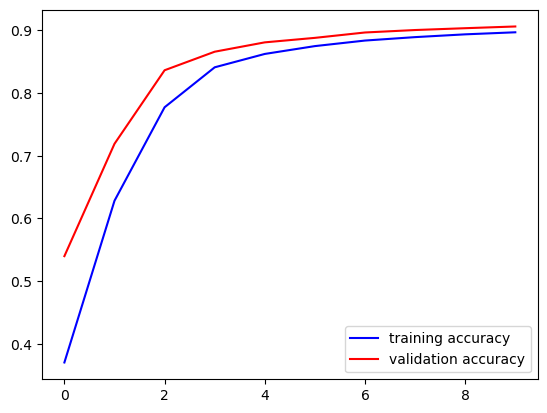
fig, ax = plt.subplots()
ax.plot(acc, '-b', label='training accuracy')
ax.plot(val_acc, '-r', label='validation accuracy')
ax.legend()
plt.show()
Evaluation and Prediction#
To get loss and metrics on the test set call Model.evaluate.
test_loss, test_metric = model.evaluate(test_images, test_labels)

test_loss, test_metric
1875/1875 ━━━━━━━━━━━━━━━━━━━━ 3s 1ms/step - categorical_accuracy: 0.9016 - loss: 0.3444
(0.3430980443954468, 0.9012500047683716)
For predictions call Model.predict.
test_pred = model.predict(test_images)
1875/1875 ━━━━━━━━━━━━━━━━━━━━ 1s 640us/step
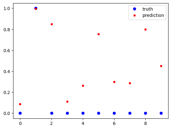
Predictions are vectors of values from \([0, 1]\). A one indicates that the image shows the corresponding digit, a zero indicates that the digits is not shown in the image.
idx = 2

print('truth:     ', test_labels[idx, :])
print('prediction:', test_pred[idx, :])

fig, ax = plt.subplots()
ax.plot(test_labels[idx, :], 'ob', label='truth')
ax.plot(test_pred[idx, :], 'or', markersize=4, label='prediction')
ax.legend()
plt.show()
truth:      [0. 1. 0. 0. 0. 0. 0. 0. 0. 0.]
prediction: [0.08869229 0.9969136  0.84936017 0.11264426 0.2628971  0.7554592
 0.29798308 0.28611335 0.79945296 0.45005688]
To get more insight into the prediction accuracy we reverse one-hot encoding.
true_digits = test_labels.argmax(axis=1)
pred_digits = test_pred.argmax(axis=1)

# indices with wrong predictions
wrong_predictions = np.arange(0, true_digits.size)[true_digits != pred_digits]
print(wrong_predictions.size)
print(wrong_predictions)
5925
[    7     8    33 ... 59974 59998 59999]
idx = 7

show_image(test_images[idx])

print('truth: {}, prediction: {}'.format(true_digits[idx], pred_digits[idx]))

truth: 9, prediction: 4
A confusion matrix depicts which digits are hard to separate for the ANN. The matrix is 10x10. The entry at row \(i\) and column \(j\) gives the number of images which show digit \(i\) (truth), but corresponding prediction is \(j\). Several Python modules provide functions for building a confusion matrix. Next to Scikit-Learn we may use Pandas for getting the matrix and Seaborn for plotting (pd.crosstab, sns.heatmap).
conf_matrix = pd.crosstab(pd.Series(true_digits, name='truth'),
                          pd.Series(pred_digits, name='prediction'))
print(conf_matrix)
prediction     0     1     2     3     4     5     6     7     8     9
truth
0           5639     1    46    17    44    74    51     7    59    14
1             11  6431    48    26    29    44    37    32   119    14
2             70    78  5237   127    50    29   219    48   162     6
3             31     2   188  5271     8   284     6    83   155    56
4             24    37    26     3  5315    10   119     2    29   215
5             83    35    27   172    92  4659    84    54   204    44
6             54    36    69     0    61    89  5626     0    22     0
7              5    38    43    27    36     7     2  5737    19   317
8             47   110    79   161    87   303    44    33  4945    81
9             20    29     6    74   184    55     2   167    83  5215
# scale values nonlinearly to get different colors at small values
scaled_conf_matrix = conf_matrix.apply(lambda x: x ** (1/2))

fig = plt.figure(figsize=(10, 8))
sns.heatmap(scaled_conf_matrix,
            annot=conf_matrix,    # use original matrix for labels
            fmt='d',    # format numbers as integers
            cmap='hot',    # color map
            cbar_kws={'ticks': []})    # no ticks for colorbar (would have scaled labels)
plt.show()

Hyperparameter Optimization#
Keras itself offers no hyperparameter optimization routines. But there is the keras-tuner module (import as keras_tuner).
import keras_tuner
We first have to create a function which builds the model and returns a Model instance. This function takes a HyperParameters object as argument containing information about hyperparameters to optimize. The build function calls methods of the HyperParameters object to get values from the current set of hyperparameters.
def build_model(hp):

    model = keras.Sequential()
    model.add(keras.Input(shape=(20, 20)))
    model.add(keras.layers.Flatten())

    layers = hp.Int('layers', 1, 3)
    neurons_per_layer = hp.Int('neurons_per_layer', 10, 40, step=10)

    for l in range(0, layers):
        model.add(keras.layers.Dense(neurons_per_layer, activation='relu'))

    model.add(keras.layers.Dense(10, activation='sigmoid'))

    model.compile(optimizer='sgd', loss='categorical_crossentropy', metrics=['categorical_accuracy'])

    return model
Now we create a Tuner object and call its search method. Several subclasses are available. RandomSearch randomly selects sets of hyperparameters and trains the model for each set of hyperparameters. The constructor takes the model building function, an objective (string with objective name of one of the model’s metrics), and the maximum number of parameter sets to test. The search function takes training and validation data in full analogy to fit.
tuner = keras_tuner.RandomSearch(build_model, 'val_categorical_accuracy', 10)
tuner.search(train_images, train_labels, validation_split=0.2, epochs=10)
Trial 10 Complete [00h 00m 26s]
val_categorical_accuracy: 0.940583348274231

Best val_categorical_accuracy So Far: 0.9538333415985107
Total elapsed time: 00h 04m 43s
Here is a summary of all models considered during hyperparameter optimization:
tuner.results_summary()
Results summary
Results in ./untitled_project
Showing 10 best trials
Objective(name="val_categorical_accuracy", direction="max")

Trial 01 summary
Hyperparameters:
layers: 3
neurons_per_layer: 40
Score: 0.9538333415985107

Trial 03 summary
Hyperparameters:
layers: 2
neurons_per_layer: 30
Score: 0.9505833387374878

Trial 07 summary
Hyperparameters:
layers: 3
neurons_per_layer: 20
Score: 0.9480000138282776

Trial 00 summary
Hyperparameters:
layers: 1
neurons_per_layer: 40
Score: 0.9437500238418579

Trial 09 summary
Hyperparameters:
layers: 1
neurons_per_layer: 30
Score: 0.940583348274231

Trial 08 summary
Hyperparameters:
layers: 2
neurons_per_layer: 20
Score: 0.9394166469573975

Trial 05 summary
Hyperparameters:
layers: 1
neurons_per_layer: 20
Score: 0.9334999918937683

Trial 04 summary
Hyperparameters:
layers: 3
neurons_per_layer: 10
Score: 0.924916684627533

Trial 02 summary
Hyperparameters:
layers: 2
neurons_per_layer: 10
Score: 0.9236666560173035

Trial 06 summary
Hyperparameters:
layers: 1
neurons_per_layer: 10
Score: 0.9185000061988831
To get the best model we may call Tuner.get_best_models, which returns a sorted (best first) list of trained Model instances. Alternatively, we may call Tuner.get_best_hyperparameters returning a list of HyperParameter objects of the best models. Based on the best hyperparameters we may train corresponding model on the full data set to improve results. Both methods take an argument specifying the number of models to return and defaulting to 1.
best_hp = tuner.get_best_hyperparameters()[0]
best_model = build_model(best_hp)
best_model.summary()
Model: "sequential_1"
┏━━━━━━━━━━━━━━━━━━━━━━━━━━━━━━━━━┳━━━━━━━━━━━━━━━━━━━━━━━━┳━━━━━━━━━━━━━━━┓
┃ Layer (type)                    ┃ Output Shape           ┃       Param # ┃
┡━━━━━━━━━━━━━━━━━━━━━━━━━━━━━━━━━╇━━━━━━━━━━━━━━━━━━━━━━━━╇━━━━━━━━━━━━━━━┩
│ flatten_1 (Flatten)             │ (None, 400)            │             0 │
├─────────────────────────────────┼────────────────────────┼───────────────┤
│ dense_2 (Dense)                 │ (None, 40)             │        16,040 │
├─────────────────────────────────┼────────────────────────┼───────────────┤
│ dense_3 (Dense)                 │ (None, 40)             │         1,640 │
├─────────────────────────────────┼────────────────────────┼───────────────┤
│ dense_4 (Dense)                 │ (None, 40)             │         1,640 │
├─────────────────────────────────┼────────────────────────┼───────────────┤
│ dense_5 (Dense)                 │ (None, 10)             │           410 │
└─────────────────────────────────┴────────────────────────┴───────────────┘
Total params: 19,730 (77.07 KB)
Trainable params: 19,730 (77.07 KB)
Non-trainable params: 0 (0.00 B)
best_model.fit(train_images, train_labels, epochs=10)
Epoch 1/10
1875/1875 ━━━━━━━━━━━━━━━━━━━━ 3s 2ms/step - categorical_accuracy: 0.6061 - loss: 1.2466
Epoch 2/10
1875/1875 ━━━━━━━━━━━━━━━━━━━━ 3s 2ms/step - categorical_accuracy: 0.9024 - loss: 0.3364
Epoch 3/10
1875/1875 ━━━━━━━━━━━━━━━━━━━━ 3s 2ms/step - categorical_accuracy: 0.9250 - loss: 0.2602
Epoch 4/10
1875/1875 ━━━━━━━━━━━━━━━━━━━━ 3s 2ms/step - categorical_accuracy: 0.9355 - loss: 0.2235
Epoch 5/10
1875/1875 ━━━━━━━━━━━━━━━━━━━━ 3s 1ms/step - categorical_accuracy: 0.9420 - loss: 0.1981
Epoch 6/10
1875/1875 ━━━━━━━━━━━━━━━━━━━━ 3s 2ms/step - categorical_accuracy: 0.9487 - loss: 0.1768
Epoch 7/10
1875/1875 ━━━━━━━━━━━━━━━━━━━━ 3s 2ms/step - categorical_accuracy: 0.9534 - loss: 0.1616
Epoch 8/10
1875/1875 ━━━━━━━━━━━━━━━━━━━━ 3s 2ms/step - categorical_accuracy: 0.9570 - loss: 0.1493
Epoch 9/10
1875/1875 ━━━━━━━━━━━━━━━━━━━━ 3s 2ms/step - categorical_accuracy: 0.9599 - loss: 0.1391
Epoch 10/10
1875/1875 ━━━━━━━━━━━━━━━━━━━━ 3s 2ms/step - categorical_accuracy: 0.9608 - loss: 0.1355
<keras.src.callbacks.history.History at 0x7ff4787662d0>
test_loss, test_metric = best_model.evaluate(test_images, test_labels)

test_loss, test_metric
1875/1875 ━━━━━━━━━━━━━━━━━━━━ 3s 2ms/step - categorical_accuracy: 0.9579 - loss: 0.1414
(0.14267222583293915, 0.9576166868209839)
Stopping Criteria#
So far we stopped training after a fixed number of epochs. But Keras also implements a mechanism for stopping training if loss or metrics stop improving. That mechanism is denoted as callbacks. We simply have to create a suitable Callback object and pass it to the fit method. Stopping criteria can be implemented with EarlyStopping objects (it’s a subclass of Callback). If we want to stop training if the validation loss starts to increase for at least 3 consecutive epochs, we have to pass monitor='val_loss', mode='min', patience=3, restore_best_weights=True. The last argument tells the fit method to not return the final model, but the best model.
es = keras.callbacks.EarlyStopping(monitor='val_loss', mode='min', patience=3, restore_best_weights=True)
best_model.fit(train_images, train_labels, validation_split=0.2, epochs=1000, callbacks=[es])
Epoch 1/1000
1500/1500 ━━━━━━━━━━━━━━━━━━━━ 3s 2ms/step - categorical_accuracy: 0.9621 - loss: 0.1266 - val_categorical_accuracy: 0.9674 - val_loss: 0.1140
Epoch 2/1000
1500/1500 ━━━━━━━━━━━━━━━━━━━━ 3s 2ms/step - categorical_accuracy: 0.9667 - loss: 0.1150 - val_categorical_accuracy: 0.9670 - val_loss: 0.1168
Epoch 3/1000
1500/1500 ━━━━━━━━━━━━━━━━━━━━ 3s 2ms/step - categorical_accuracy: 0.9668 - loss: 0.1119 - val_categorical_accuracy: 0.9657 - val_loss: 0.1186
Epoch 4/1000
1500/1500 ━━━━━━━━━━━━━━━━━━━━ 3s 2ms/step - categorical_accuracy: 0.9686 - loss: 0.1068 - val_categorical_accuracy: 0.9676 - val_loss: 0.1128
Epoch 5/1000
1500/1500 ━━━━━━━━━━━━━━━━━━━━ 3s 2ms/step - categorical_accuracy: 0.9703 - loss: 0.1027 - val_categorical_accuracy: 0.9654 - val_loss: 0.1165
Epoch 6/1000
1500/1500 ━━━━━━━━━━━━━━━━━━━━ 3s 2ms/step - categorical_accuracy: 0.9711 - loss: 0.0982 - val_categorical_accuracy: 0.9665 - val_loss: 0.1110
Epoch 7/1000
1500/1500 ━━━━━━━━━━━━━━━━━━━━ 3s 2ms/step - categorical_accuracy: 0.9730 - loss: 0.0934 - val_categorical_accuracy: 0.9679 - val_loss: 0.1150
Epoch 8/1000
1500/1500 ━━━━━━━━━━━━━━━━━━━━ 3s 2ms/step - categorical_accuracy: 0.9731 - loss: 0.0915 - val_categorical_accuracy: 0.9675 - val_loss: 0.1129
Epoch 9/1000
1500/1500 ━━━━━━━━━━━━━━━━━━━━ 3s 2ms/step - categorical_accuracy: 0.9742 - loss: 0.0872 - val_categorical_accuracy: 0.9650 - val_loss: 0.1117
<keras.src.callbacks.history.History at 0x7ff47df04b30>
Resulting accuracy on test set:
test_loss, test_metric = best_model.evaluate(test_images, test_labels)
test_loss, test_metric
1875/1875 ━━━━━━━━━━━━━━━━━━━━ 3s 2ms/step - categorical_accuracy: 0.9627 - loss: 0.1232
(0.12472119927406311, 0.962233304977417)
Saving and Loading Models#
Keras models provide a save method to save a model to a file. To load a model use load_model.
best_model.save('keras_save_best_model.keras')
model = keras.models.load_model('keras_save_best_model.keras')
Visualization of Training Progress#
TensorFlow comes with a visualization tool called TensorBoard. It uses a web interface for visualizing training dynamics and it can be integrated into Jupyter notebooks.
To use TensorBoard we have to pass a TensorBoard callback to fit. Corresponding constructor takes a path to a directory for storing temporary training data. Running
tensorboard --logdir=path/to/directory
in the terminal will show an URL to access the TensorBoard interface within a web browser.
To use TensorBoard inside a Jupyter Notebook, execute the magic commands
%load_ext tensorboard
%tensorboard --logdir path/to/directory
es = keras.callbacks.EarlyStopping(monitor='val_loss', mode='min', patience=3, restore_best_weights=True)
tb = keras.callbacks.TensorBoard('tensorboard_data')
best_model.fit(train_images, train_labels, validation_split=0.2, epochs=1000, callbacks=[es, tb])
Epoch 1/1000
1500/1500 ━━━━━━━━━━━━━━━━━━━━ 4s 3ms/step - categorical_accuracy: 0.9729 - loss: 0.0929 - val_categorical_accuracy: 0.9659 - val_loss: 0.1180
Epoch 2/1000
1500/1500 ━━━━━━━━━━━━━━━━━━━━ 4s 3ms/step - categorical_accuracy: 0.9718 - loss: 0.0917 - val_categorical_accuracy: 0.9659 - val_loss: 0.1123
Epoch 3/1000
1500/1500 ━━━━━━━━━━━━━━━━━━━━ 4s 3ms/step - categorical_accuracy: 0.9727 - loss: 0.0892 - val_categorical_accuracy: 0.9652 - val_loss: 0.1157
Epoch 4/1000
1500/1500 ━━━━━━━━━━━━━━━━━━━━ 4s 2ms/step - categorical_accuracy: 0.9748 - loss: 0.0797 - val_categorical_accuracy: 0.9667 - val_loss: 0.1126
Epoch 5/1000
1500/1500 ━━━━━━━━━━━━━━━━━━━━ 4s 2ms/step - categorical_accuracy: 0.9769 - loss: 0.0782 - val_categorical_accuracy: 0.9652 - val_loss: 0.1160
<keras.src.callbacks.history.History at 0x7ff47df50770>
%load_ext tensorboard
%tensorboard --logdir tensorboard_data