Bernoulli-Verteilung

Definition

Eine Bernoulli-Verteilung liegt vor, wenn eine Zufallsvariable nur zwei verschiedene Werte annehmen kann.

Definition

Sei \(0\leq p\leq 1\). Die Zufallsvariable \(X\) heißt Bernoulli-verteilt, falls sie entsprechend Tabelle

Wert \(x\)	\(0\)	\(1\)
\(\mathbb P(X=x)\)	\(1-p\)	\(p\)

verteilt ist. Wir schreiben dann kurz:

\[X\sim \mathrm{Ber}(p)\]

Anwendung

Typische Anwendungsszenarien:

• Münzwurf

• Qualitätskontrolle: defekt, nicht defekt

• Klinische Studien: krank, gesund

• Zielschuss: treffen, nicht treffen

• usw. (immer wenn ein Zufallsexperiment genau 2 mögliche Ausgänge gibt)

Eigenschaften

Gilt \(X\)

Erwartungswert:

\[\mathbb E(X)= 0\cdot (1-p) + 1\cdot p = p \]

Varianz:

\[\mathrm{Var}(X)= \mathbb E(X^2)-\mathbb E(X)^2 =0^2\cdot (1-p) + 1^2\cdot p - p^2 = p-p^2=p(1-p) \]

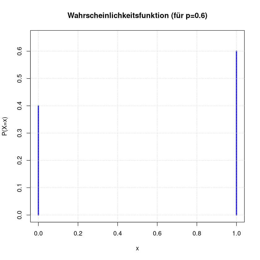
Stabdiagramm:

Show code cell source Hide code cell source

x     <- c(0,1)
probs <- c(0.4,0.6)

plot(x = x, y = probs, col = "blue", type = "h", lwd = 3,ylim=c(0,0.65), 
     main = "Wahrscheinlichkeitsfunktion (für p=0.6)", ylab = "P(X=x)", xlab = "x")
grid()

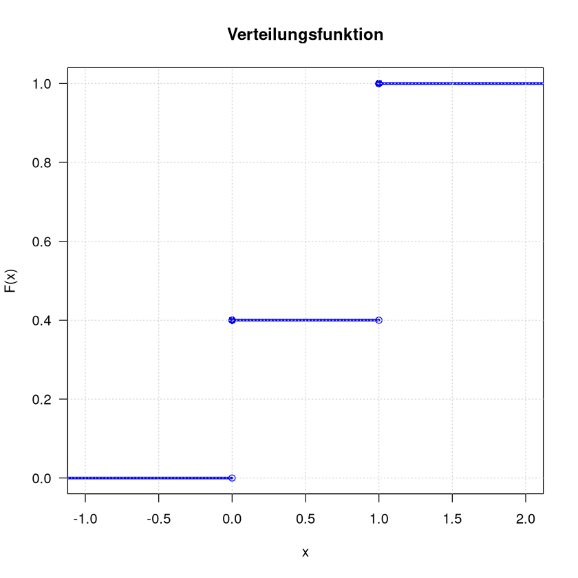
Verteilungsfunktion

\[\begin{split}F:\mathbb R\to\mathbb R,\qquad F(x)= \begin{cases}0 & \text{falls } x<0\\ 0.4 & \text{falls } 0\leq x < 1 \\ 1 & \text{falls } x \geq 1 \end{cases}\end{split}\]

Show code cell source Hide code cell source

plot.dcdf <- function(x, prob , col="blue", lwd=3, ...) {
  y   <- c(0,cumsum(prob))
  cdf <- stepfun(x=x, y=y, right=TRUE)
  plot(cdf, verticals=FALSE,
       lwd=lwd, col=col, las=1, 
       xlab="x", ylab="F(x)", ...)
  points(x,cumsum(prob),pch = 16, col=col, cex=1.2)
}
plot.dcdf(c(0,1), c(0.4,0.6), main="Verteilungsfunktion")
grid()

Beispiel

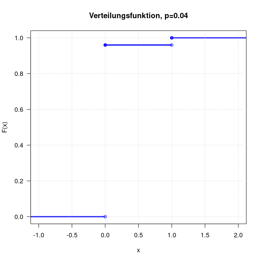
Der Ausschussanteil in einer Produktion liege bei \(4\%\). Wir greifen zufällig ein Teil aus der laufenden Produktion heraus. Die Zufallsvariable die das modelliert ist \(X\sim\mathrm{Ber}(0.04)\).

Es gilt also \(\mathbb P(X=0)=0.96\) und \(\mathbb P(X=1)=0.04\) und

\[\mathbb E(X) = 0.04\quad \text{ und }\quad \mathrm{Var}(X)=0.04\cdot 0.96 = 0.0384\]

Die Standardabweichung: \(\sqrt{\mathrm{Var}(X)} = 0.195959\)

Verteilungsfunktion:

Show code cell source Hide code cell source

plot.dcdf(c(0,1), c(0.96,0.04), main="Verteilungsfunktion, p=0.04")
grid()